ANOVA

What ANOVA does

ANalysis Of VAriance
do multiple (more than 2) populations have the same mean?
different types of variance are used to figure this out (sums of squares)
null hypothesis: all groups do have the same mean
alternative hypothesis: at least one mean differs from the others
a low p-value means that the null is rejected, i.e. that at least one mean differs significantly
functions: aov() ; oneway.test ; …

Assumptions

data points must be independent
all populations must be (approximately) normally distributed
exploring normality: same as for T-test (with all groups)
all groups must have similar variance (homoscedasticity)

Some data:

file.exists("anova_data.txt")

## [1] TRUE

df = read.table("anova_data.txt", header = FALSE)
colnames(df)

## [1] "V1" "V2" "V3" "V4"

colnames(df) = c("A", "B", "C", "D")
head(df)

##             A        B          C          D
## 1  0.35304697 4.983129  1.7420254  3.4038870
## 2 -0.92555558 4.479949  1.0426776 -1.1661505
## 3  1.47636942 4.054450 -1.8529604  0.5629787
## 4 -0.65262182 3.926977  0.5773551  1.7024414
## 5  0.87934474 5.626965  1.2850280  3.6237300
## 6  0.02417173 2.180872  1.2049257  0.6112000

A boxplot (or violin plot) can help to get a first impression. Do the groups overlap?

boxplot(df, col="green", main="Comparison of four datasets")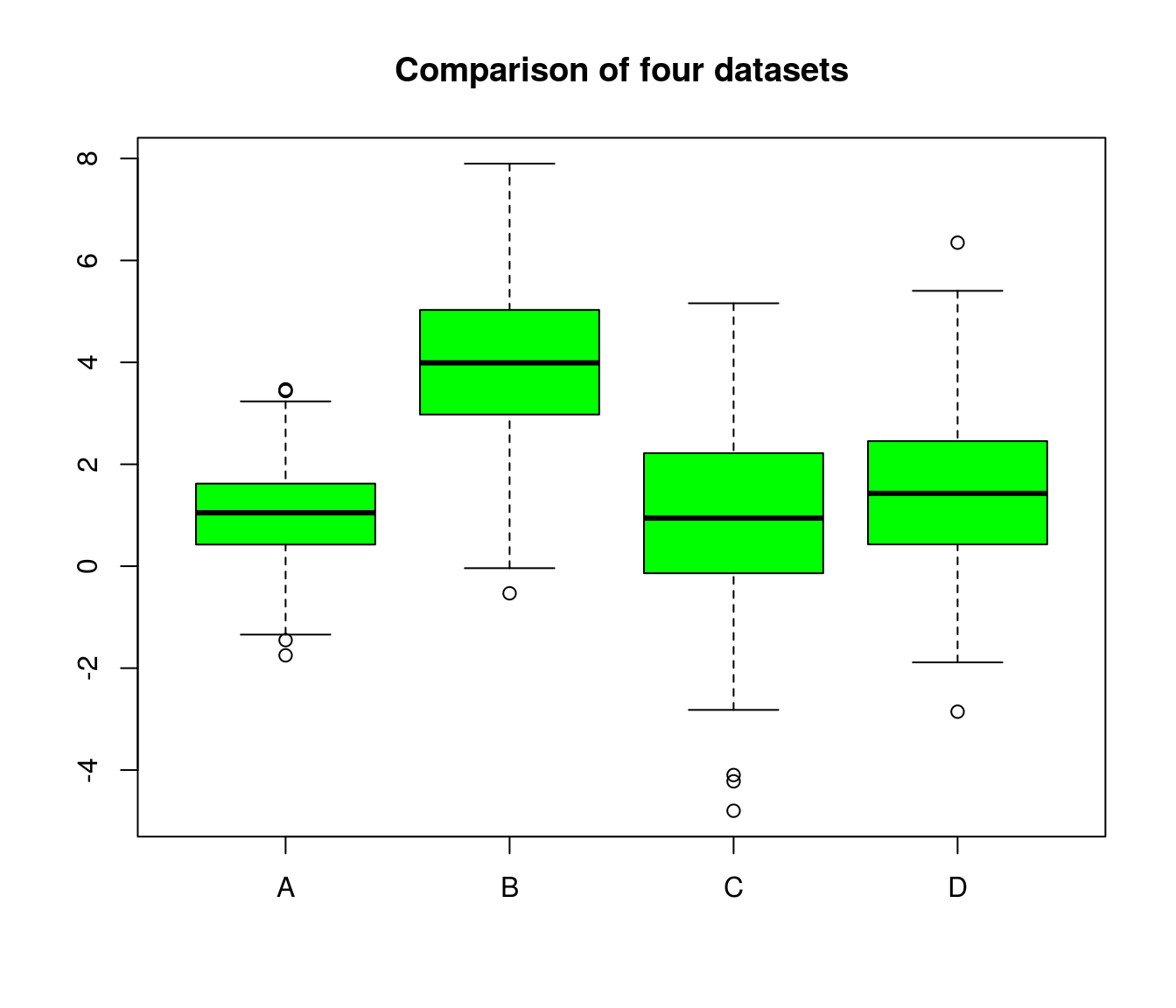

summary(df)

##        A                 B                 C                 D          
##  Min.   :-1.7489   Min.   :-0.5317   Min.   :-4.7983   Min.   :-2.8548  
##  1st Qu.: 0.4257   1st Qu.: 2.9825   1st Qu.:-0.1313   1st Qu.: 0.4384  
##  Median : 1.0482   Median : 3.9907   Median : 0.9446   Median : 1.4285  
##  Mean   : 1.0204   Mean   : 3.9939   Mean   : 0.9602   Mean   : 1.4527  
##  3rd Qu.: 1.6174   3rd Qu.: 5.0288   3rd Qu.: 2.2157   3rd Qu.: 2.4535  
##  Max.   : 3.4694   Max.   : 7.8987   Max.   : 5.1594   Max.   : 6.3481

suppressMessages(library(vioplot))    # load library silently  
vioplot(df$A, df$B, df$C, df$D, col = "gold", names = c("g1", "g2", "g3", "g4"))
title("Comparison of four groups", font.main = 1)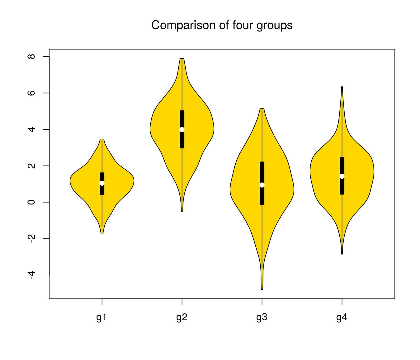

Checking for homoscledasticity

Look at the boxplot!
use bartlett.test (but might be significant for large datasets, even if the differences are small)

Running the ANOVA using `aov()`

Some functions (e.g. aov() need stacked data as input:

stacked <- stack(df)
colnames(stacked) <- c("values", "groups")
head(stacked)

##        values groups
## 1  0.35304697      A
## 2 -0.92555558      A
## 3  1.47636942      A
## 4 -0.65262182      A
## 5  0.87934474      A
## 6  0.02417173      A

tail(stacked)

##          values groups
## 1195  3.5114304      D
## 1196  1.1461898      D
## 1197 -0.5427561      D
## 1198  2.3259909      D
## 1199  1.4033644      D
## 1200  0.5924236      D

str(stacked)

## 'data.frame':    1200 obs. of  2 variables:
##  $ values: num  0.353 -0.926 1.476 -0.653 0.879 ...
##  $ groups: Factor w/ 4 levels "A","B","C","D": 1 1 1 1 1 1 1 1 1 1 ...

Running aov():

Low p-values: \(H_0\) to be rejected –> at least one mean differs significantly

res <- aov(values ~ groups, data = stacked)  
summary(res)   # reject the null

##               Df Sum Sq Mean Sq F value Pr(>F)    
## groups         3   1870   623.4     303 <2e-16 ***
## Residuals   1196   2461     2.1                   
## ---
## Signif. codes:  0 '***' 0.001 '**' 0.01 '*' 0.05 '.' 0.1 ' ' 1

Which group differs?

run post-hoc test
Tukey’s HSD (Honest Significant Difference)
the Tukey test automatically corrects for multiple testing in a smart way

tuk <- TukeyHSD(res)
tuk

##   Tukey multiple comparisons of means
##     95% family-wise confidence level
## 
## Fit: aov(formula = values ~ groups, data = stacked)
## 
## $groups
##            diff        lwr        upr     p adj
## B-A  2.97345793  2.6721526  3.2747632 0.0000000
## C-A -0.06021073 -0.3615160  0.2410946 0.9557379
## D-A  0.43228489  0.1309796  0.7335902 0.0013327
## C-B -3.03366865 -3.3349740 -2.7323633 0.0000000
## D-B -2.54117303 -2.8424783 -2.2398677 0.0000000
## D-C  0.49249562  0.1911903  0.7938009 0.0001644

plot(tuk)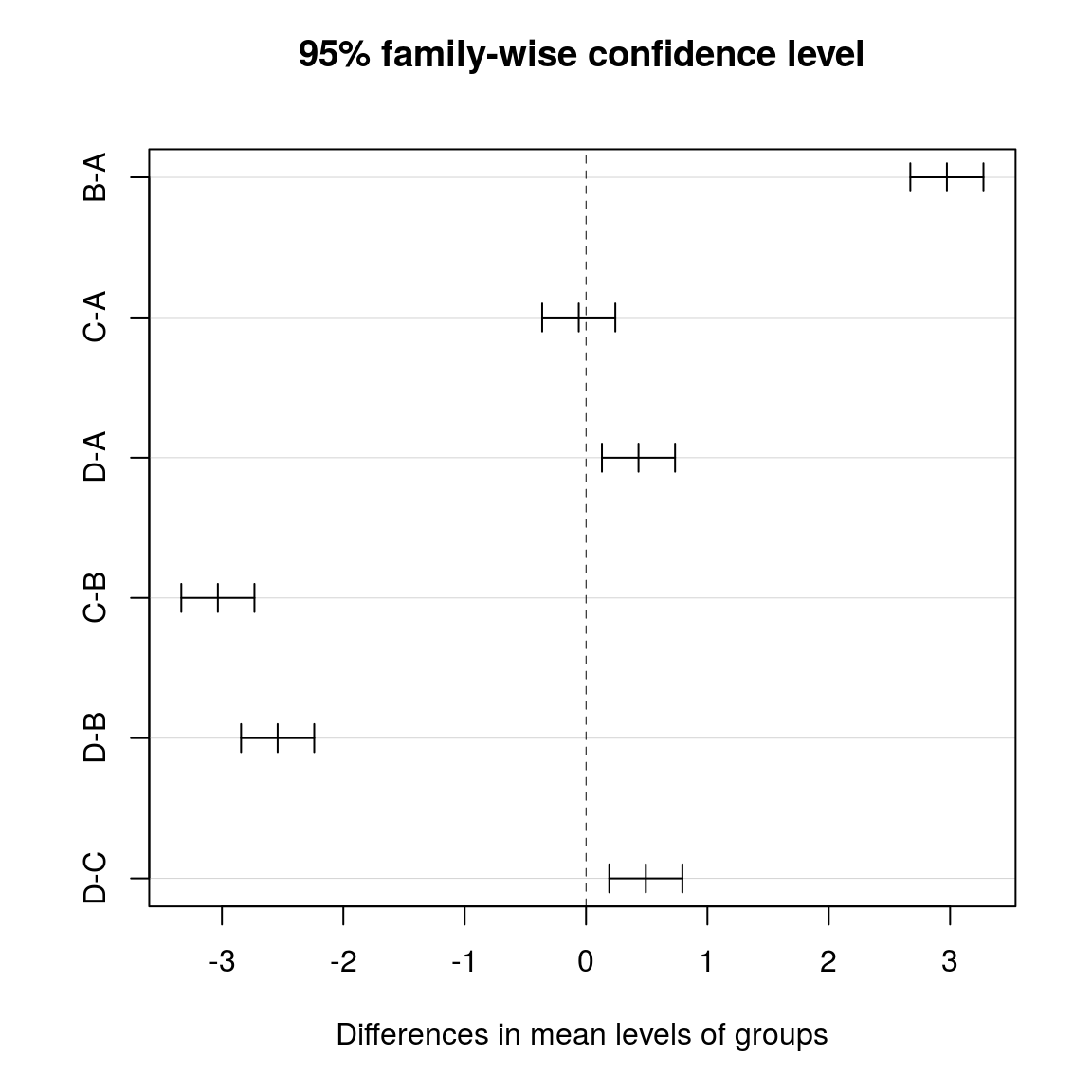

Running the ANOVA using `oneway.test()`

Which one to choose?

oneway.test() can correct for nonhomogeneity of the variances (Welch correction)
no post hoc test available for oneway.test()

data(InsectSprays)                                  # get some R dataset
head(InsectSprays)

##   count spray
## 1    10     A
## 2     7     A
## 3    20     A
## 4    14     A
## 5    14     A
## 6    12     A

str(InsectSprays)

## 'data.frame':    72 obs. of  2 variables:
##  $ count: num  10 7 20 14 14 12 10 23 17 20 ...
##  $ spray: Factor w/ 6 levels "A","B","C","D",..: 1 1 1 1 1 1 1 1 1 1 ...

levels(InsectSprays$spray)                          # 6 levels

## [1] "A" "B" "C" "D" "E" "F"

boxplot(count ~ spray, data = InsectSprays)         # not normally distr. (assymmetric), different variance in the groups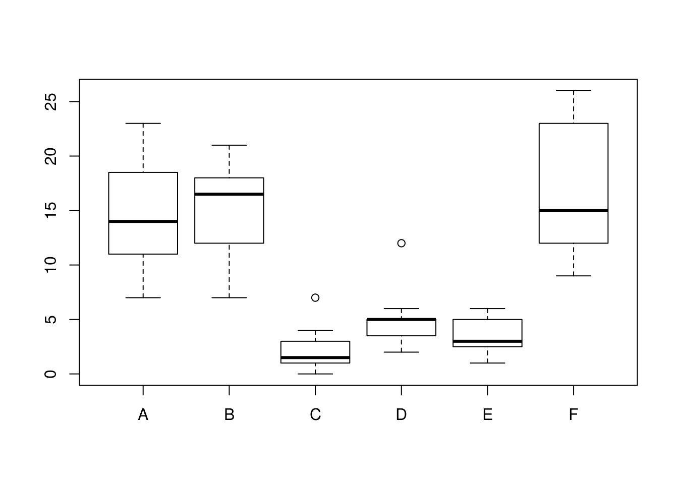

bartlett.test(count ~ spray, data = InsectSprays)   # check for heteroscedasticity

## 
##  Bartlett test of homogeneity of variances
## 
## data:  count by spray
## Bartlett's K-squared = 25.96, df = 5, p-value = 9.085e-05

oneway.test(count ~ spray, data = InsectSprays)     # var.equal = FALSE is default!

## 
##  One-way analysis of means (not assuming equal variances)
## 
## data:  count and spray
## F = 36.065, num df = 5.000, denom df = 30.043, p-value = 7.999e-12

When the assumptions for ANOVA are not met, part I

Try data tranformation? (log, square root, …)

The same as for T-test

When the assumptions for ANOVA are not met, part II

Conduct a non-parametric test (rank sum test)

Kruskal-Wallis test
rank-based nonparametric test
if the data is normally distributed, the ANOVA is better (has more power)

kruskal.test(df)                               # on data frame

## 
##  Kruskal-Wallis rank sum test
## 
## data:  df
## Kruskal-Wallis chi-squared = 480.82, df = 3, p-value < 2.2e-16

kruskal.test(values ~ groups, data = stacked)  # on stacked data

## 
##  Kruskal-Wallis rank sum test
## 
## data:  values by groups
## Kruskal-Wallis chi-squared = 480.82, df = 3, p-value < 2.2e-16