The package phangorn
What can `phangorn’ do?
- Functions for the construction of phylogenetic trees and networks
- CRAN site (with several vignettes)
- R documentation chapter
- Paper
- Quick and dirty tree building in R
Reading multiple alignments into R
library(phangorn)
options(width = 140)
# help(phangorn)
primates <- read.phyDat("primates.dna", format = "phylip")  # from one the vignettes coming with pahangorn
class(primates)
## [1] "phyDat"names(primates)## [1] "Mouse" "Bovine" "Lemur" "Tarsier" "Squir Monk" "Jpn Macaq" "Rhesus Mac" "Crab-E.Mac" "BarbMacaq" "Gibbon"
## [11] "Orang" "Gorilla" "Chimp" "Human"print(primates)## 14 sequences with 232 character and 217 different site patterns.
## The states are a c g tlength(primates)## [1] 14image(primates)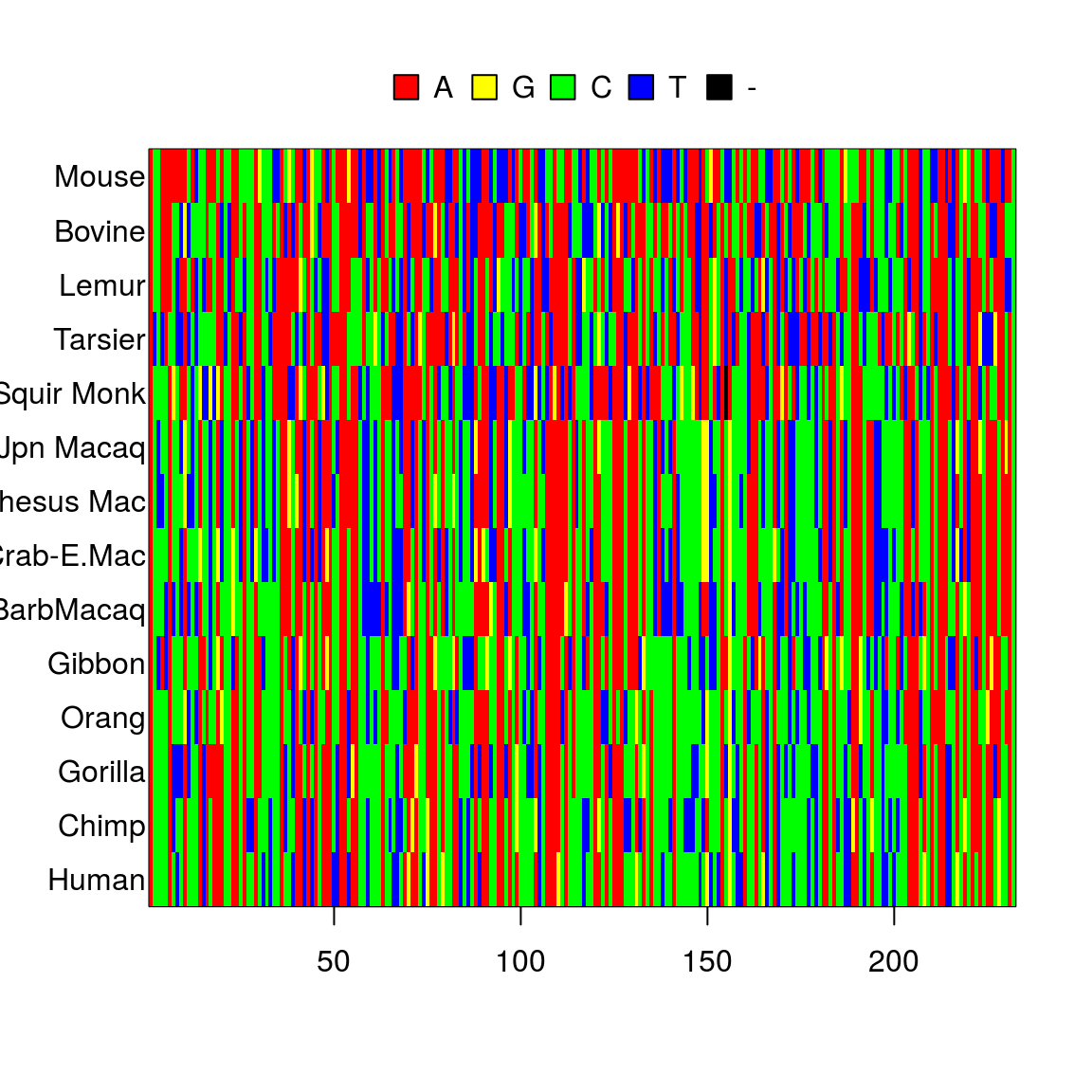
df <- as.data.frame(primates)
dim(df)
## [1] 232 14head(df)## Mouse Bovine Lemur Tarsier Squir Monk Jpn Macaq Rhesus Mac Crab-E.Mac BarbMacaq Gibbon Orang Gorilla Chimp Human
## 1 a a a a a a a a a a a a a a
## 2 c c c t c c c c c c c c c c
## 3 c c c c c t t c c t c c c c
## 4 a a a t c c t c c a c c c c
## 5 a a a a c c c c t t c c c c
## 6 a a a c a a a a a a a a a aaln1 <- as.MultipleAlignment(primates)
class(aln1) # can be done a lot now using Biostrings library## [1] "DNAMultipleAlignment"
## attr(,"package")
## [1] "Biostrings"Plotting a phylogenetic tree
The functions ‘dist.hamming’, ‘dist.ml’ and ‘dist.logDet’ compute pairwise distances for an object of class ‘phyDat’. THe function ‘dist.ml’ uses DNA or AA sequences to compute distances under different substitution models.
distance <- dist.ml(primates)
class(distance)
## [1] "dist"length(distance)## [1] 9114*13/2## [1] 91treeNJ = NJ(distance)
class(treeNJ)## [1] "phylo"print(treeNJ)##
## Phylogenetic tree with 14 tips and 12 internal nodes.
##
## Tip labels:
## Mouse, Bovine, Lemur, Tarsier, Squir Monk, Jpn Macaq, ...
##
## Unrooted; includes branch lengths.Nedge(treeNJ)## [1] 25Nnode(treeNJ) ## [1] 12plot(treeNJ)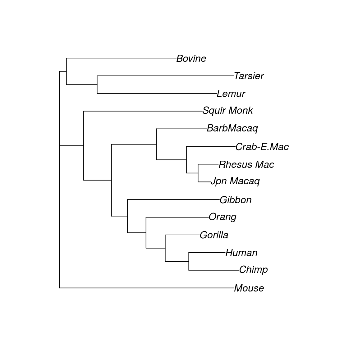
plot(treeNJ, "unrooted", main="Neighbor joining tree", font.main = 1)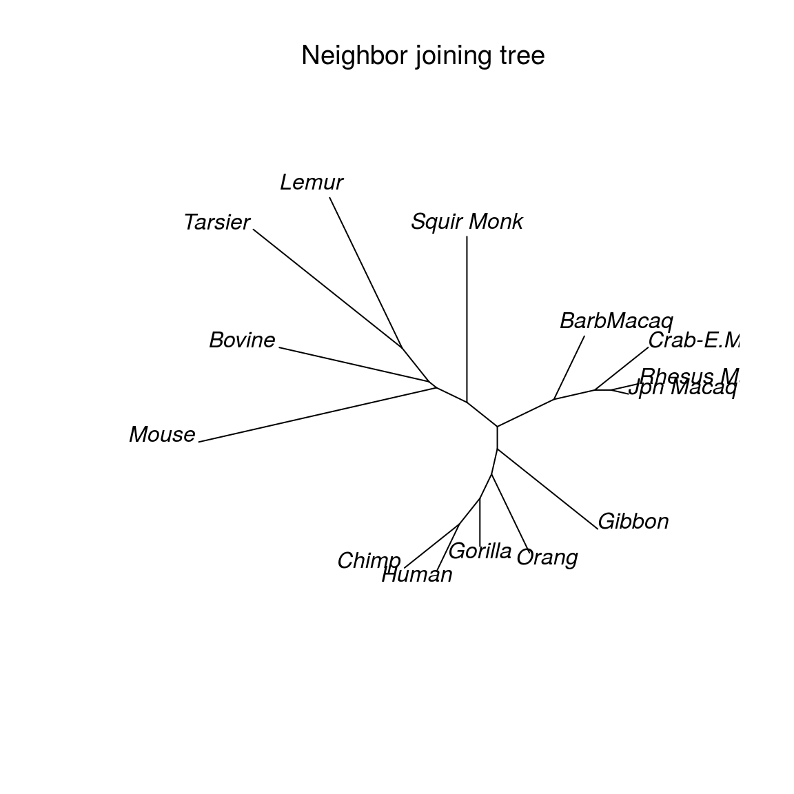
treeUPGMA <- upgma(distance)
plot(treeUPGMA)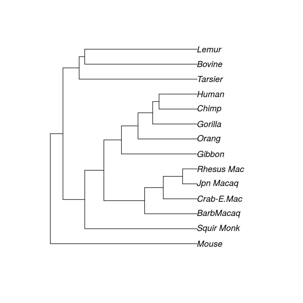
Parsimony and likelihood for a tree
The best hypothesis is the one that requires the fewest evolutionary changes. The function parsimony return the parsimony score for a given alignment.
parsimony(treeUPGMA, primates) ## [1] 751fit <- pml(treeNJ, data = primates)
fit##
## loglikelihood: -3074.952
##
## unconstrained loglikelihood: -1230.335
##
## Rate matrix:
## a c g t
## a 0 1 1 1
## c 1 0 1 1
## g 1 1 0 1
## t 1 1 1 0
##
## Base frequencies:
## 0.25 0.25 0.25 0.25fitJC <- optim.pml(fit, TRUE)## optimize edge weights: -3074.952 --> -3068.417
## optimize edge weights: -3068.417 --> -3068.417
## optimize topology: -3068.417 --> -3068.295
## optimize topology: -3068.295 --> -3068.295
## 1
## optimize edge weights: -3068.295 --> -3068.295
## optimize topology: -3068.295 --> -3068.295
## 0
## optimize edge weights: -3068.295 --> -3068.295fitJC ##
## loglikelihood: -3068.295
##
## unconstrained loglikelihood: -1230.335
##
## Rate matrix:
## a c g t
## a 0 1 1 1
## c 1 0 1 1
## g 1 1 0 1
## t 1 1 1 0
##
## Base frequencies:
## 0.25 0.25 0.25 0.25