T-test
What the test does
- are two populations having the same mean?
- null hypothesis: the groups do have the same mean
- a low p-value means that the null is rejected, i.e. that the means are significantly different
Assumptions
- data points must be independent
- both populations must be (approximately) normally distributed
# Testing normality of samples:
sets <- read.table("set1_set2.csv", header=TRUE)    # read from disk and store in variable (object) "sets"
set1 = sets[,1]                                     # 1st column
set2 = sets[,2]                                     # 2nd column
# Histogram:
hist(set1, col = "red", breaks = 20)                # does it approximately resemble a normal distribution?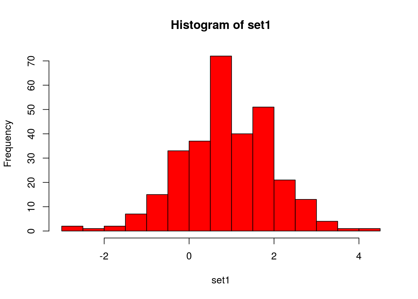
# Quantile-quantile plot:
qqnorm(set1, col = "blue")
qqline(set1, col = "red")                           # data points should be close to the line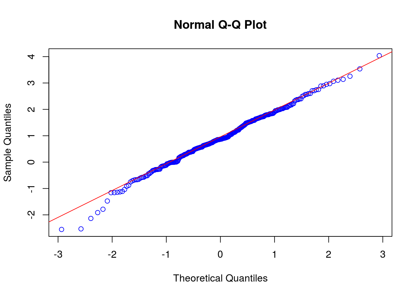
# Tests:
# Kolmogorow-Smirnow-Test. Null: data is normally distributed. Big p-values are desired!
ks.test(set1, "pnorm", mean(set1), sd(set1))
##
## One-sample Kolmogorov-Smirnov test
##
## data: set1
## D = 0.035656, p-value = 0.8402
## alternative hypothesis: two-sided# Shapiro-Wilk normality test. Null: data is normally distributed. Big p-values are desired! No standardisation necessary.
shapiro.test(set1)##
## Shapiro-Wilk normality test
##
## data: set1
## W = 0.99367, p-value = 0.2415# Anderson-Darling test.
library(nortest)
ad.test(set1)##
## Anderson-Darling normality test
##
## data: set1
## A = 0.41021, p-value = 0.3412Running the test
A boxplot (or violin plot) can help to get a first impression. Do the gropus overlap?
boxplot(sets, col="green", names=c("set1", "set2"), main="Comparison of two datasets")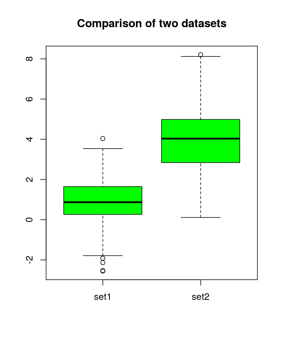
The simplest form of the command ‘t.test’:
?t.test
t.test(set1, set2)
##
## Welch Two Sample t-test
##
## data: set1 and set2
## t = -28.436, df = 527.39, p-value < 2.2e-16
## alternative hypothesis: true difference in means is not equal to 0
## 95 percent confidence interval:
## -3.275339 -2.852041
## sample estimates:
## mean of x mean of y
## 0.8987499 3.9624399If the variances are similar, it might be better to set the parameter ‘var.equal’ to TRUE:
t.test(set1, set2, var.equal = TRUE)##
## Two Sample t-test
##
## data: set1 and set2
## t = -28.436, df = 598, p-value < 2.2e-16
## alternative hypothesis: true difference in means is not equal to 0
## 95 percent confidence interval:
## -3.275282 -2.852098
## sample estimates:
## mean of x mean of y
## 0.8987499 3.9624399One-sided tests can be made:
t.test(set1, set2, alternative = "less")##
## Welch Two Sample t-test
##
## data: set1 and set2
## t = -28.436, df = 527.39, p-value < 2.2e-16
## alternative hypothesis: true difference in means is less than 0
## 95 percent confidence interval:
## -Inf -2.886164
## sample estimates:
## mean of x mean of y
## 0.8987499 3.9624399t.test(set1, set2, alternative = "greater")##
## Welch Two Sample t-test
##
## data: set1 and set2
## t = -28.436, df = 527.39, p-value = 1
## alternative hypothesis: true difference in means is greater than 0
## 95 percent confidence interval:
## -3.241216 Inf
## sample estimates:
## mean of x mean of y
## 0.8987499 3.9624399The confidence level (\(1 - \alpha\)) can be changed:
t.test(set1, set2, conf.level = 0.99)##
## Welch Two Sample t-test
##
## data: set1 and set2
## t = -28.436, df = 527.39, p-value < 2.2e-16
## alternative hypothesis: true difference in means is not equal to 0
## 99 percent confidence interval:
## -3.342214 -2.785166
## sample estimates:
## mean of x mean of y
## 0.8987499 3.9624399A test for paired samples can be conducted:
x = seq(1, 10)
y = x + 2 + rnorm(length(x), mean = 0, sd = 0.3)
plot(x, ylim = c(min(x,y), max(x,y)), col = "red", main = "Paired data", font.main = 1)
points(y, col = "blue")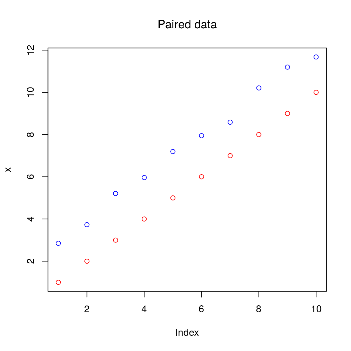
t.test(x, y, paired = TRUE)##
## Paired t-test
##
## data: x and y
## t = -25.705, df = 9, p-value = 9.831e-10
## alternative hypothesis: true difference in means is not equal to 0
## 95 percent confidence interval:
## -2.127913 -1.783680
## sample estimates:
## mean of the differences
## -1.955796When the assumptions are not met, part I
Try data tranformation? (log, square root, …)
file.exists("setb.txt")## [1] TRUEsetb <- read.table("setb.txt", header = FALSE)
setb <- setb[,1] # convert from data.fram to numeric
is.numeric(setb)## [1] TRUElength(setb)## [1] 300# Normally distributed?:
hist(setb, col = "red", breaks = 20)![]()
qqnorm(setb, col = "blue")
qqline(setb, col = "red")![]()
shapiro.test(setb) ##
## Shapiro-Wilk normality test
##
## data: setb
## W = 0.65755, p-value < 2.2e-16# Transform and repeat check for normality:
setb_trans = log(setb)
hist(setb_trans, col = "red", breaks = 20)![]()
qqnorm(setb_trans, col = "blue")
qqline(setb_trans, col = "red")![]()
shapiro.test(setb_trans)##
## Shapiro-Wilk normality test
##
## data: setb_trans
## W = 0.99266, p-value = 0.1471# Ready for the T-test:
t.test(set1, setb_trans)##
## Welch Two Sample t-test
##
## data: set1 and setb_trans
## t = -0.77151, df = 597.99, p-value = 0.4407
## alternative hypothesis: true difference in means is not equal to 0
## 95 percent confidence interval:
## -0.2341234 0.1020581
## sample estimates:
## mean of x mean of y
## 0.8987499 0.9647825When the assumptions are not met, part II
Conduct a non-parametric test (rank sum test)
Many different names for the same (ranksum) test:
- Mann–Whitney U test
- Mann–Whitney–Wilcoxon test
- Wilcoxon rank-sum test
- Wilcoxon–Mann–Whitney test
- Wikipedia
x = runif(200, 0, 1)
y = runif(200, 2, 3)
boxplot(x, y, col = "green")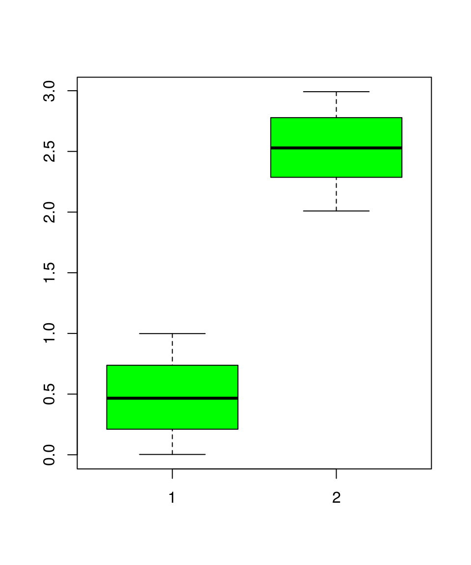
wilcox.test(x, y)##
## Wilcoxon rank sum test with continuity correction
##
## data: x and y
## W = 0, p-value < 2.2e-16
## alternative hypothesis: true location shift is not equal to 0